In my first post of the year I will provide a gentle introduction to web scraping with the tidyverse package rvest. As the package name pun suggests, web scraping is the process of harvesting, or extracting, data from websites. The extraction process is greatly simplified by the fact that websites are predominantly built using HTML (= Hyper Text Markup Language), which essentially uses a set of formatting and structuring rules to tell your browser how to display a website. By navigating the website structure and requesting the desired formatting element (e.g. a certain image, hyperlink, or bold-face text) we can scrape the underlying information. With more and more information stored online, web scraping is a valuable tool in your data science tool box. There’s not much background required to understand this post, other than dplyr basics and a bit of HTML.
This post will also provide a throwback to my former life as astronomer. The dataset we will scrape is related to an ongoing long-term project of observing a fascinating exploding star in our neighbour galaxy Andromeda. Our star is one of a kind: it belongs to the class of Novae and erupts roughly once a year - much more frequently than any other nova.
The dataset is publicly available in the archives of NASA’s Neil Gehrels Swift Observatory. Fun fact: all data of publicly funded astronomical observatories (e.g. from all NASA or ESA telescopes) is freely available to anyone (due to that very public funding); sometimes immediately after it was taken, sometimes a year or so later to give the observing team a head start. Lots of discovery space out there.
To begin, as usual we load the required packages first:
libs <- c('dplyr', 'tibble',      # wrangling
          'stringr', 'rvest',     # strings, scraping
          'knitr', 'kableExtra',  # table styling
          'lubridate', 'ggplot2') # time, plots
invisible(lapply(libs, library, character.only = TRUE))
This is the link for the page we’re starting with:
target_link <- "https://www.swift.ac.uk/swift_portal/getobject.php?name=m31n+2008-12a&submit=Search+Names"We know that our star has the prosaic catalogue name “M31N 2008-12a” (or at least I still know that name in my sleep), so this is what we will plug into the search name syntax of the UK Swift Science Data Centre. Below is the result:
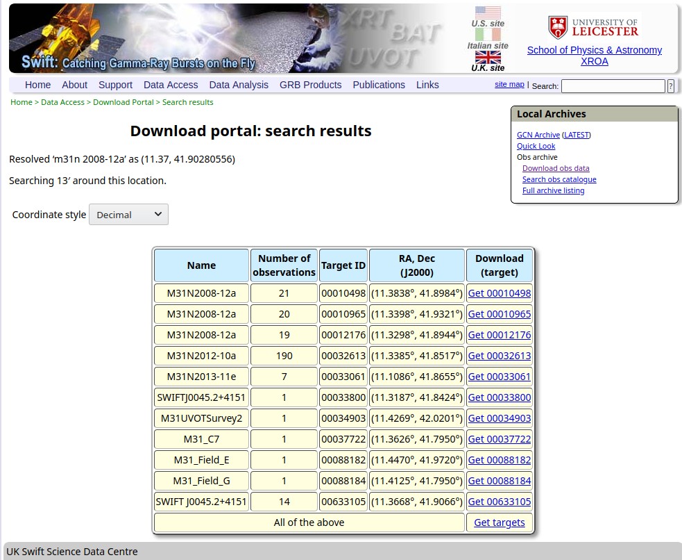
Search result for M31N 2008-12a
Among some other elements, this page has a prominent table which contains all Swift observations that covered the position of our object on the sky. As you see, not all of those were pointed at M31N 2008-12a; some serendipitous observations featured our explosive friend somewhere near the edge of the field of view. But we’re not picky, we take all we can get. We download the entire page using the read_html tool and store it in the variable target_page. This might take a moment or two:
target_page <- read_html(target_link)The result isn’t very pretty, yet. It just shows us the HTML header and the HTML body and a whole lot of text and formatting associated with it. (I’m not showing it here because the output confuses some rss readers.)
Luckily, we don’t have to mess around with the HTML text in this unstructured form. In order to find out exactly which element we need, we can use the Inspector tool of our browsers. Chances are, you just need to press F12 to launch it.
Now you should see something like this, with the Inspector tool taking up part of the screen. The Inspector window (here on the right) shows the HTML code of the website in the upper half of the window (plus some stuff we don’t care about in this post in the lower half):
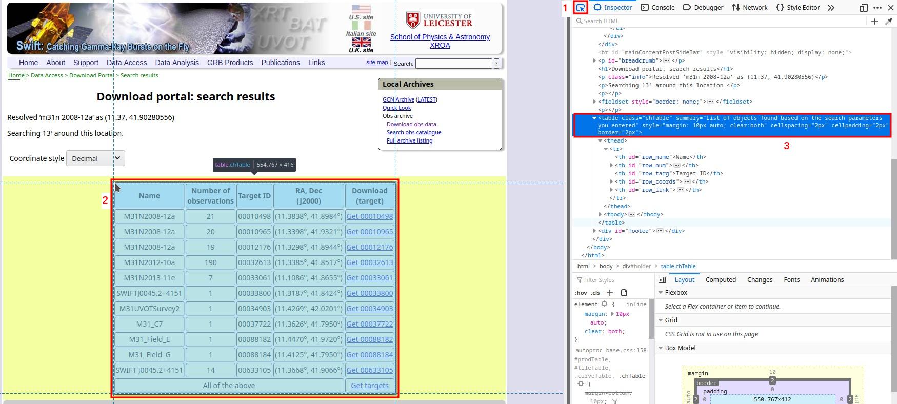
Website with Inspector tool
To identify the path for the element we need (here the big table) we will go through the following 3 steps, which I’ve marked in the image above:
Click on the arrow in the top left corner of the Inspector window to get the element picker [1].
Go to the website window and position your mouse pointer so that the selection mask covers the entire element you’re interested in, but not more [2]. In the image above, my mouse pointer masks the entire table with a blue shade but doesn’t select “Coordinate style” or the “Local Archives” box on the top right. (Ignore the yellow shade; there are no elements there.) Once you’re happy with the selection confirm it with a left click.
Upon clicking, the Inspector code window will automatically navigate to the selected element and highlight it in blue [3]. Now all you have to do is go anywhere on that blue background, do a right click, and select “Copy -> XPath”. In our case, the result is
/html/body/div/table. This is the path that navigates through the HTML hierarchy to our table.
Now we can use the tool html_nodes to extract the element. This gives us the HTML code; including the formatting. Because it is a table, we then use html_table to extract only the table itself. Other extraction tools include html_text or html_form. This great tutorial by Ryan Thomas contains a list of the various extraction functions (and much more).
The rest of the code cell below turns the table into a tidy tibble and does a bit of formatting. Then we print the result:
target <- target_page %>%
  html_nodes(xpath = "/html/body/div/table") %>%
  html_table()

target <- target[[1]] %>%
  as_tibble() %>%
  rename(target = Name,
         num_obs = `Number of observations`,
         target_id = `Target ID`,
         coords = `RA, Dec (J2000)`) %>%
  select(-`Download(target)`) %>%
  filter(target != "All of the above")

target %>%
  select(-coords) %>%
  kable() %>%
kable_styling()| target | num_obs | target_id |
|---|---|---|
| M31N2008-12a | 21 | 00010498 |
| M31N2008-12a | 20 | 00010965 |
| M31N2008-12a | 19 | 00012176 |
| M31N2012-10a | 190 | 00032613 |
| M31N2013-11e | 7 | 00033061 |
| SWIFTJ0045.2+4151 | 1 | 00033800 |
| M31UVOTSurvey2 | 1 | 00034903 |
| M31_C7 | 1 | 00037722 |
| M31_Field_E | 1 | 00088182 |
| M31_Field_G | 1 | 00088184 |
| SWIFT J0045.2+4151 | 14 | 00633105 |
As you can easily confirm we successfully extracted the entire table. Note: since this is an ongoing project and our star subject is prone to roughly yearly eruptions you can expect some of these numbers to change within less than a year from now (Jan 2020). Some stellar evolutions take billions of years, some are in a bit more of a hurry.
But enough poetry - what have we actually done here? Well, the interesting part of the exercise was extracting the target_id values. You see: each position or object that Swift observes in the sky gets its own unique target ID; and sometimes even more than one (for internal housekeeping reasons). In order to get all the information about the 21 or 19 or 190 individual observations associated with a target ID we need to query a second website with these very same IDs.
Before that: a quick primer on scraping best practices: first and foremost: respect the wishes and resources of the server. This means don’t overwhelm the server with lots of scraping requests in a very short time. Besides being rather impolite, such high-frequency requests will likely get your IP blocked. Most websites list the rules for scrapers and other bots in their robots.txt file (e.g. twitter). Some sites may disallow scraping entirely. As always: be kind.
So this first exercise was primarily a preparation for building the following link:
obsid_link_prefix <- "https://www.swift.ac.uk/archive/selectseq.php?tid="
obsid_link_suffix <- "&source=obs&name=m31n%202008-12a&reproc=1"

obsid_link_targets <- target %>%
  mutate(target_id = str_sub(target_id, start = 4)) %>%
  pull(target_id) %>%
  str_c(collapse = ",")

obsid_link <- str_c(obsid_link_prefix,
                    obsid_link_targets,
                    obsid_link_suffix)

obsid_link
## [1] "https://www.swift.ac.uk/archive/selectseq.php?tid=10498,10965,12176,32613,33061,33800,34903,37722,88182,88184,33105&source=obs&name=m31n%202008-12a&reproc=1"You see that the link contains all the target_id values that we just scraped from the big table. Following this link gets us to an even bigger table which lists all the individual observations for each target_id together with some meta data. From that page, we could even directly download the data and start playing with it.
For now, we will follow the exact same strategy as above: we scrape the page, extract the table using its XPath, turn it into a tidy tibble, and apply some slight adjustments. If you feel like doing a mini challenge then try to find the relevant XPath (or even build the entire extraction) without looking at the code below.
# download the data
obsid_page <- read_html(obsid_link)

# copy the xpath from the site's html, extract table
obsid <- obsid_page %>%
  html_nodes(xpath = '/html/body/div/form/div/div[3]/table') %>%
  html_table()

# table is first element, turn into tibble
obsid <- obsid[[1]] %>%
  as_tibble(.name_repair = "unique")

# change names, remove rows for download all of 1 target ID
obsid <- obsid %>%
  select(-...1) %>%
  rename(obsid = ObsID,
         hea_ver = `HEASoft Ver`,
         start_time = `Start time (UT)`,
         exp_xrt = `XRT exposure (s)`) %>%
  filter(!str_detect(hea_ver, "000")) %>%
  select(-hea_ver) %>%
  mutate(obsid = str_c("000", as.character(obsid))) %>%
  mutate(target_id = str_sub(obsid, 4, 8))
And those are the first 5 rows:
obsid %>%
  head(5) %>%
  kable() %>%
kable_styling()| obsid | start_time | exp_xrt | target_id |
|---|---|---|---|
| 00010498001 | 2018-01-01T05:07:09 | 990.4 | 10498 |
| 00010498002 | 2018-01-02T08:26:27 | 995.4 | 10498 |
| 00010498003 | 2018-01-03T19:20:57 | 682.0 | 10498 |
| 00010498004 | 2018-01-04T11:31:57 | 1271.2 | 10498 |
| 00010498005 | 2018-01-05T11:22:57 | 5218.7 | 10498 |
We now have an ObsID, which uniquely identifies each observation, the start date & time of the observation, the target_id from the previous table (which is part of the obsid), and also exp_xrt: the exposure time of Swift’s X-ray Telescope. This exposure time measures how long the X-ray detector of the telescope was exposed to light from the star. Units are in seconds.
Another fun fact: X-ray astronomers like me love it to measure (exposure) time in kilo seconds (ks), i.e. \(10^3~s\). This could be considered the ultimate triumph of the metric system (who needs minutes or hours anyway?), but then we’d also use weird units like erg or, and I kid you not, Crab. So, overall it’s probably a tie when it comes to the progress of metric units … .
Anyway, here’s some plots on what that data we just scraped tells us about the X-ray observations. First, the number of observations per year up to now:
foo <- obsid %>%
  mutate(start_date = date(start_time)) %>%
  mutate(year = as.integer(year(start_date)),
         month = month(start_date, label = TRUE, abbr = TRUE))

foo %>%
  count(year) %>%
  ggplot(aes(year, n, fill = n)) +
  geom_col() +
  geom_label(aes(label = n), col = "black") +
  scale_fill_viridis_c(option = "viridis",
                       begin = 0.5, end = 0.9) +
  theme(legend.position = "none") +
  scale_x_continuous(breaks = seq(min(foo$year),
                                  max(foo$year), 1)) +
  labs(x = "Year", y = "Number of observations",
       caption = "The M31N 2008-12a monitoring collaboration") +
  ggtitle("Neil Gehrels Swift Observatory coverage of nova M31N 2008-12a",
          subtitle = "Targeted observations began in 2013. In 2015 we conducted the\nX-ray flash monitoring campaign. In 2017 the eruption happened on NYE.")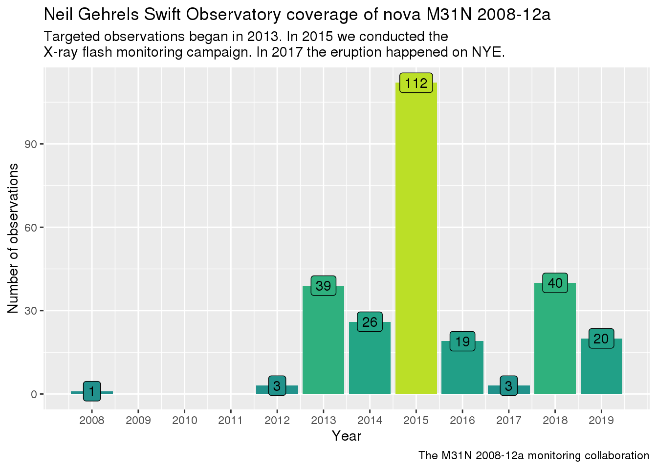
Observations prior to 2013 did not detect the eruptions; in 2013 our targeted campaign began. 2015 was an odd year, because we were running a separate high-frequency campaign trying to catch an elusive X-ray flash, which had never been observed in any object. Unfortunately, it still hasn’t. In 2017 the eruption had the nerves to happen on New Year’s Eve, so almost all observations happened in early 2018 (and our NYE parties briefly got a bit hectic). The 2020 eruption will probably happen in October, but don’t bet too much money on it.
If you look at cumulative exposure time instead of number of observations you see that in 2015 most of those 112 observations were much shorter than usual:
foo %>%
  group_by(year) %>%
  summarise(exp_xrt = sum(exp_xrt)/1e3) %>%
  ggplot(aes(year, exp_xrt, fill = exp_xrt)) +
  geom_col() +
  #geom_label(aes(label = n), col = "black") +
  scale_fill_viridis_c(option = "magma",
                       begin = 0.5, end = 0.9) +
  theme(legend.position = "none") +
  scale_x_continuous(breaks = seq(min(foo$year),
                                  max(foo$year), 1)) +
  labs(x = "Year", y = "Combined XRT Exposure [ks]",
       caption = "The M31N 2008-12a monitoring collaboration") +
  ggtitle("Neil Gehrels Swift Observatory coverage of nova M31N 2008-12a")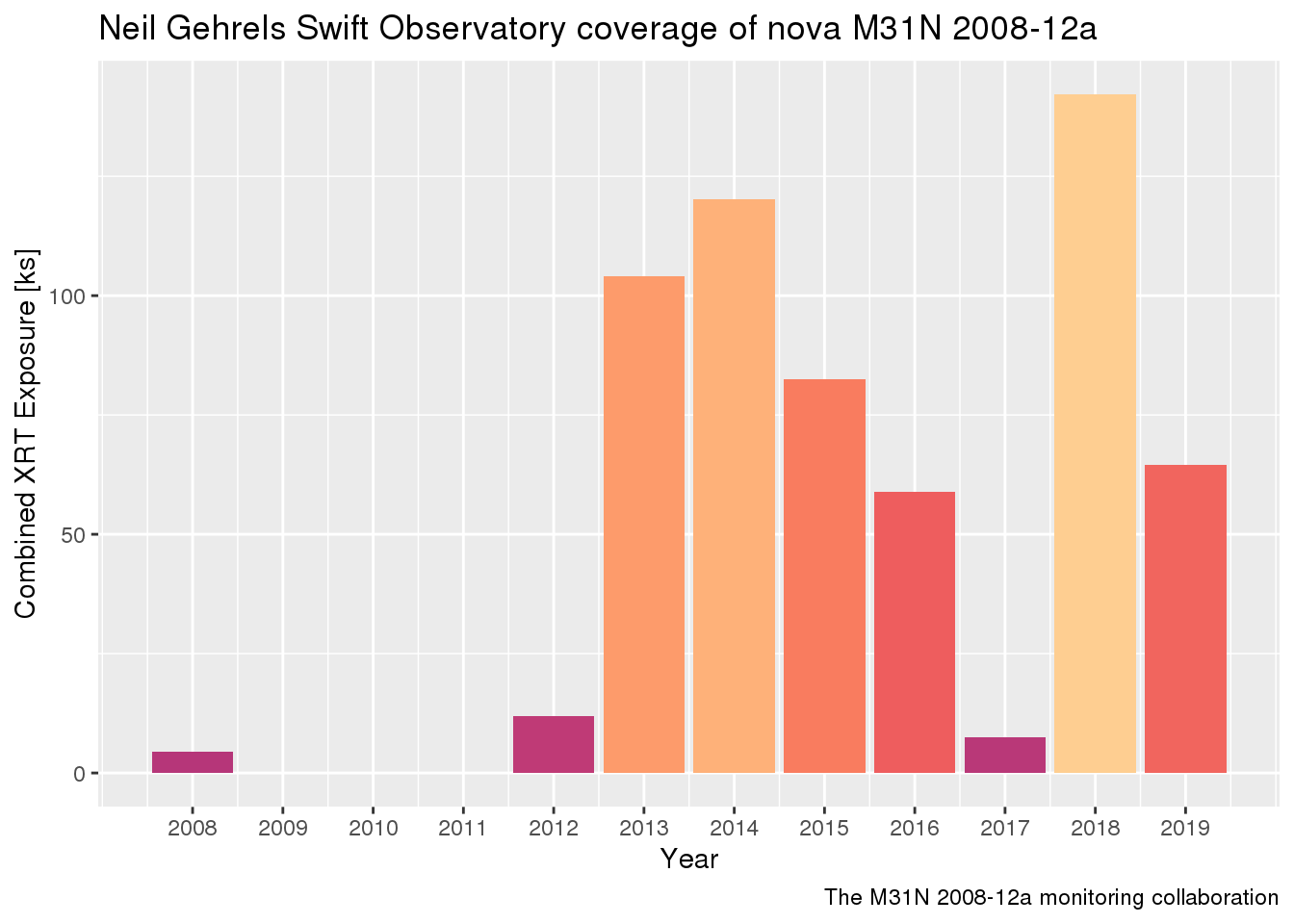
Up to Jan 2020, we have used Swift to look at M31N 2008-12a in the X-rays for a total of almost exactly 600 ks. Which is more than half a mega second. Now that’s an impressive unit. Coincidentally, with Rstudio::conf 2020 coming up in San Francisco next week, my next post might happen within the next mega second. Watch this space ;-)
More info:
While rvest works great for static websites, sometimes you encounter pages that are built dynamically or require interaction like filling in a form or clicking a button. In those cases, Rselenium is the right tool. I might do a post on it in the future.
Shout-out to my good friend and colleague Matt Darnley, together with whom I built and led this astro project for several years and who continues to do exciting work at the frontiers of astrophysics. He’s a great person to follow if you want to learn more about exploding stars.
If you’re interested you can also check out our recent Nature publication, led by Matt, for another highlight produced by the mercurial nova M31N 2008-12a.
If you are an astronomy enthusiast and want to contribute to cutting edge research on variable stars, here’s my advice: join the international AAVSO. Whether you have a telescope, some binoculars, or no instruments at all; they have tons of advice on how anyone can get involved in variable star astronomy.