Tidy evaluation in R - Simple Examples

The tidyverse philosophy introduced by Hadley Wickham has been a game changer for the R community. It is based on intuitive rules of what a tidy data set should look like: each variable is a column, each observation is a row (Wickham 2014). At its core, the tidyverse collection of R packages is powered by a consistent grammar of data manipulation and visualisation.

The tidyverse grammar makes it easier to manipulate data sets using simple expressions that reduce the syntactic overhead and allow you to focus on the data. Thus, packages like dplyr or tidyr are great for exploratory data analysis (EDA) and hands-on data wrangling. A small downside of this approach is that these tools require a bit more effort when using them in functions with variable parameters. In general you want to use functions to improve the reusability and reproducibility of your code.

This is where the tidy evaluation comes in. A few additional methods and concepts are sufficient to make all your tidy code run smoothly in a function context. Here I will go through some relatively simple examples to get you started.

Before we begin we will need the following libraries:

libs <- c('dplyr', 'tibble',              # wrangling
          'datasets',                     # data
          'knitr','kableExtra',           # table styling
          'ggplot2','gridExtra')          # plots, panels
invisible(lapply(libs, library, character.only = TRUE))

We will use the Orange data set, which is part of the datasets package and records the growth of 5 orange trees. Here are the first 5 rows:

Tree	age	circumference
1	118	30
1	484	51
1	664	75
1	1004	108

Personally, I’m learning most efficiently by first looking at examples that show the code in action and then tweaking them to fit my needs. After playing with the code for a bit and inevitably breaking something I turn to the docs to understand more about the syntax and additional arguments of the function. Thus, all my posts on tools or methodology will follow the same pattern: I will jump right into the action by looking at a useful yet simple example or two. Next, I dissect this example, maybe break something, and explain the arguments. In closing, there will be a few more complex examples, caveats, pointers, and/or resources. Sounds good? Here we go:

The first example is a function that takes as input a data frame df and a variable var from that data frame (i.e. a column/feature). The output is the difference between the (global) median and the mean of the variable. This is a realistic example of a concise helper function, since it goes beyond basic in-built tools and provides a quick check on whether a distribution is symmetric¹:

median_minus_mean <- function(df, var){
  
  var <- enquo(var)
  
  df %>% 
    summarise(foo = median(!!var) - mean(!!var)) %>% 
    .$foo
}

Now we apply it to the circumference of trees to find that the mean is larger than the median:

median_minus_mean(Orange, circumference)

## [1] -0.8571429

To understand how it works here are the 2 key concepts:

• Quoting: In the body of the function, the variable var is being quoted by the enquo function (borrowed from the rlang package). This essentially means that the content (or argument) of the variable is being encoded. The quotation stops this variable from being immediately evaluated. Instead, its content is being treated as a functional R expression.

• Unquoting: In order to tell a tidyverse verb like summarise that you are passing it the content of a quoted variable you need to unquote it. Practically you are copy-pasting the variable expression into the verb. This is done using the !! operator which Hadley wants to be pronounced bang-bang. I can only surmise that he said that because it makes boring conversations about code sound like wild-west movie fights.

In most situations enquo and !! are all you need. Conceptually, there’s a bit more to it since enquo encodes the current state of the environment along with the variable. This is a useful property, which makes enquo aware of parameters defined outside a function, but for now you can ignore these finer details.

(Talking about details: foo or bar are popular names for dummy variables in many programming languages. It’s just something that needs a name for the moment but can immediately be forgotten once its time-limited purpose is fulfilled.)

Also: yes, this works:

median_minus_mean <- function(df, var){
  df %>% 
    summarise(foo = median(!!enquo(var)) - mean(!!enquo(var))) %>% 
    .$foo
}
median_minus_mean(Orange, circumference)

## [1] -0.8571429

You can quote and unquote in the same step. Let’s go a bit further and include grouping by another variable, here the age of the trees:

median_minus_mean <- function(df, var, gvar){
  
  var <- enquo(var)
  gvar <- enquo(gvar)
  
  df %>% 
    group_by(!!gvar) %>% 
    summarise(foo = median(!!var) - mean(!!var)) %>% 
    .$foo
}

median_minus_mean(Orange, circumference, age)

## [1] -1.0  0.2 -6.2 -9.2 -3.6  0.6  1.2

Turns out that for some ages the mean circumference is smaller than the median.

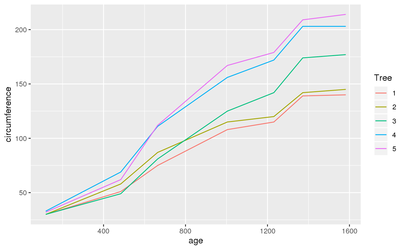
Good news: quote/unquote also works for ggplot2. Here we quote the x, y, and colour-group variables of our plot:

plot_growth_tree <- function(df, xvar, yvar, gvar){
  
  xvar <- enquo(xvar)
  yvar <- enquo(yvar)
  gvar <- enquo(gvar)
  
  df %>% 
    ggplot(aes(!!xvar, !!yvar, col = !!gvar)) +
    geom_line()
}

plot_growth_tree(Orange, age, circumference, Tree)

Some trees grow faster than others.

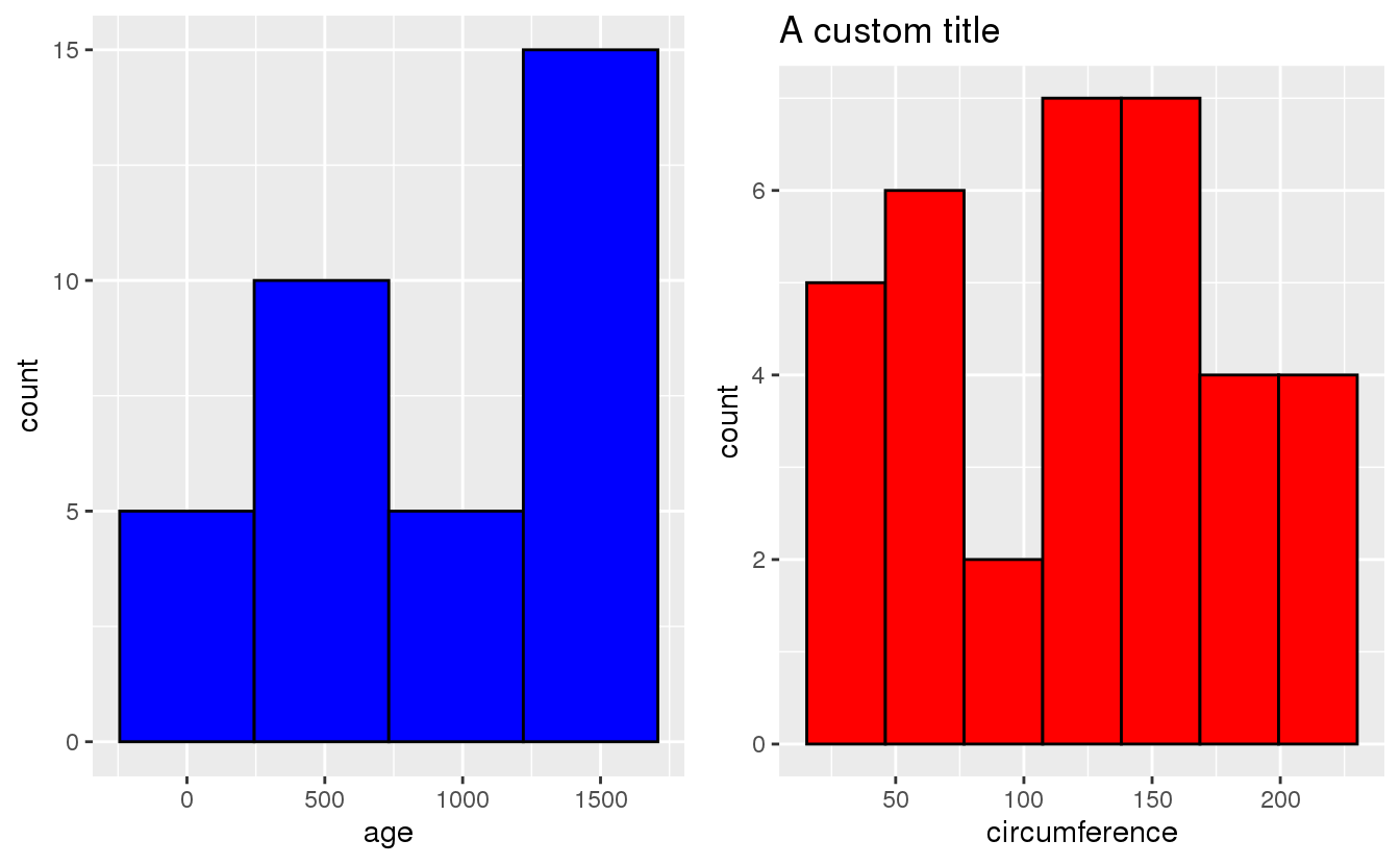
In fact, ggplot2 is a great use case because it allows us to quickly built helper functions if we need to repeat a certain plot for many similar features. Individual modification to those templates can be added using the ggplot2 grammar. Here is a histogram example where we add a custom title to the second plot²:

plot_hist <- function(df, var, bins, bcol){
  
  var <- enquo(var)
  
  df %>% 
    ggplot(aes(!!var)) +
    geom_histogram(bins = bins, fill = bcol, col = "black")
}

p1 <- plot_hist(Orange, age, 4, "blue")
p2 <- plot_hist(Orange, circumference, 7, "red") +
  ggtitle("A custom title")

grid.arrange(p1, p2, layout_matrix = rbind(c(1,2)))

You see that here the number of histogram bins and the plot colour are being passed to the function as normal integer and string - without need of being quoted. This works because these parameters are not R expressions.

There will be a second post soon about more complex tidy evaluation examples. If you’re interested, watch this space.

In the meantime: Curious about the bigger picture?

• The tidy evaluation book is a great starting guide into the concepts.

• This thread collects some typical use cases for tidy evaluation.

• For a concise 5 minute intro to the main concepts by the man himself watch Hadley here: